Skydiving Math

Introduction

I must admit that I was amazed at what Felix Baumgartner accomplished. As I watched the video, I found myself focusing on the video's display of Felix's speed versus time. It was really interesting to see how he quickly he accelerated to faster than Mach 1 speed and then he began to decelerate as he hit denser atmosphere. The video below is the one I was watching.

As I thought about, I could compare Felix's speed versus time data with the predictions from a differential equation. This gives me another opportunity to try out Mathcad Prime 2.0. Let's dig in ...

Background

My approach to this problem is simple:

• Capture the empirical data from the jump video and put it into Mathcad Prime.

  This was the only routine and boring part of the exercise.

• Capture data from NASA on the atmosphere's density and the variation in gravity with altitude.

  I used this same file for my post on Mars's atmosphere.

• Create a differential equation model and use Mathcad Prime to solve it.

  I will use the high-speed drag model shown in the Wikipedia to keep things simple. I have used a more sophisticated drag model in a previous blog post, but I wanted to keep this one simple. Since Felix was spinning and changing position, his coefficient of drag was changing -- modeling it as a constant is sure to be wrong. I am just looking for an approximate model. However, it may provide some insight into what was going on.

• Tune the differential equation model's coefficient of drag (defined below) to best match the empirical data

  I am constantly performing optimizations at work. I might as well start getting used to optimizations in Mathcad Prime.

• Compare the empirical data to the tuned differential equation model and see how well the mathematics compares to reality.

  Here is where I get practice with the graphics in Mathcad Prime.

Analysis

Empirical Speed Capture

My approach to capturing the speed data was simple.

• Watch this video.
• Write down the numbers for times and speeds that I see on the video.

I am afraid sometimes you just have to sit there and write stuff down by hand. There are problems with gathering the data this way.

• The data is quantized in one second intervals.
• Sometimes the data changes two or three times during a single one second interval.
• The speed data may also be quantized -- the speed numbers are not changing continuously.

What this means is that the data I took by hand suffers from quantization errors (both in amplitude and timing). To minimize these errors, I will both smooth and interpolate the my rough speed and time readings.

Figure 1 shows how the data looks in Mathcad Prime 2 after I did my post-processing.

Modeling Atmospheric Density and Gravity

This data comes straight from NASA and all I am doing is running the data through an interpolation routine. Figure 2 shows how this interpolation looks in Mathcad Prime.

Atmospheric Drag Modeling

The skydiver experiences two forces during his fall:

• atmospheric drag
• gravity

These two forces are combined into a single differential equation. Let's first review the effects of both drag and gravity.

The Wikipedia has a very good discussion of drag for those readers requiring more background. I will use Equation 1 from this article to model the force of drag on the skydiver.

Eq. 1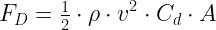

where

• F_D is the force of drag [N]
• A is the cross-sectional area presented to the air stream [m²]
• ρ(x) is the density of the atmosphere as a function of altitude [kg/m³] -- from here
• C_D is the coefficient of drag [unitless]
• v is the velocity of the skydiver [m/s]

Gravity Modeling

Modeling the force of gravity is simpler than modeling drag, but we will increase the complexity just a tad by incorporating its variation with altitude. While this is a small effect, it does provide for a more complete model. Equation 2 shows the mathematical model I will be using.

Eq. 2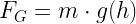

where

• m is the mass of the skydiver and equipment [kg]
• g(h) is the acceleration due to gravity as a function of height [m/s²]

I will use a guess for the mass of the skydiver (m=100 kg), and I will obtain the gravitational acceleration as a function of height from this document.

Overall Differential Equation

With both drag and gravity modeled, we can now write down the full differential equation (Equation 3).

Eq. 3

With this equation, we can now setup our differential equation solver, which I show in Figure 3.

Optimizing My Estimate for the Coefficient of Drag

I have no idea what the coefficient of drag is for a skydiver wearing a pressure suit. I will use an optimization routine to determine the coefficient of drag that best matches the empirical speed data. Figure 4 shows how this optimizer was setup.

Results

Figure 5 shows the comparison between my mathematical model and the empirical speed data.

Conclusion

The empirical data and the output of the mathematical model are very similar. At this point, I think I understand the modeling. It really is remarkable how good a simple model can be. The exercise also proved to be a good exercise in the use of Mathcad Prime 2.0.

Appendix A: Mathcad Source File

Here is the Mathcad Prime 2.0 file that was used to make this blog post.
Skydiving.mcdx
This is an XML file. Just download it to your desktop and open it up with Mathcad. For those without Mathcad, here is the PDF version.
Skydiver.pdf