Battery Failure Rates and Continuously-Compounded Interest

Quote of the Day

The man who does not read good books has no advantage over the man who cannot read them.

— Mark Twain

Introduction

Figure 1: A Common Sealed Lead Acid Battery.

While performing some routine reliability analysis, I noticed that there is a similarity between battery aging and continuously-compounded interest calculations. I had not noticed this similarity before, and I thought I would document it here.

Figure 1 shows a common lead-acid battery. This chemistry is my focus in this post. Other chemistries will behave similarly, but the constants involved will differ. I will be assuming that the failure rate of the battery is described by the Arrhenius equation.

Background

To understand this post, we need to establish a bit of knowledge in two areas:

Chemical Reaction Rates and the Arrhenius Equation
Continuously Compounded Interest

Chemical Reaction Rates and the Arrhenius Equation

Batteries are chemical machines and their performance is predictable using the mathematics of chemical kinetics. For our purposes here, the key equation is the Arrhenius Equation, which I state in Equation 1.

Eq. 1

$\displaystyle k=A\cdot {{e}^{-\frac{{{E}_{a}}}{R\cdot T}}}$

where

A is a reaction-dependent constant.
My work here will involve only relative values, which means that the exact value of A will not be important.
T is the absolute temperature.
A common calculation error is to work in celsius and not Kelvin. Make sure that all your battery work is in Kelvin.
E_a is the activation energy.
The primary corrosion reaction has an activation energy of about 50 kilo-Joules (kJ) per mole (reference).
R is the universal gas constant.

The Wikipedia has a very good article on the Arrhenius equation. I have also reviewed the Arrhenius equation in earlier post, and I will assume those in need of further review will venture there.

Continuously Compounded Interest

The Wikipedia provides some good background on continuously compounded interest. I will review the mathematics behind continuous compounding briefly here.

Equation 2 shows the basic compound interest formula.

Eq. 2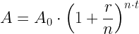

$\displaystyle A=A_0 \cdot {{\left( 1+\frac{r}{n} \right)}^{n \cdot t}}$

where

A is the final value of the investment (principal and interest)
A₀ is the principal amount (initial investment)
r is the annual nominal interest rate
n is number of times the interest is compounded per year
t is number of years the investment receives interest payments

Assume that we want to compute the interest paid after one year (t = 1) to an account where the interest is compounded an infinite number of times (n = ?). Equation 3 shows the basic steps in the derivation.

Eq. 3

${{A}_{\infty }}=\underset{n\to \infty }{\mathop{\lim }}\,\ {{A}_{0}}\cdot {{\left( 1+\frac{r}{n} \right)}^{n\cdot t}}={{A}_{0}}\cdot {{e}^{r\cdot t}}$

where

A_? is the final value of the investment after infinitely many compounding cycles.

Assume we are interested in the amount of time required to double our investment assuming continuous compounding. Equation 4 illustrates that computation.

Eq. 4

$\displaystyle 2\cdot A=A\cdot {{e}^{r\cdot t}}\Rightarrow t=\frac{\ln (2)}{r}$

This equation is related to the famous "Rule of 72", which makes calculations of investment doubling time simple enough to do in your head (see here and here). It turns out that Equation 4 is also useful in computing the temperature increase required to halve the life of a battery.

Analysis

Battery Longevity's Relationship to Chemical Reaction Rates

The battery's longevity is determined by the speed of the corrosion reaction -- a faster corrosion reaction will corrode the battery faster and bring its demise sooner. No wonder why the concept of passivation is essential for metal. Not everyone is going to understand this topic in particular, but through companies such as astropak, you can learn even more about what the process of passivation involves. You learn something new everyday.
We can derive the impact of this faster corrosion reaction on the battery's lifetime by making a couple of assumptions:

The battery is considered failed when its capacity has been reduced below the level needed to provide adequate backup capacity.
In the telcom industry, we normally consider a battery to have failed when its backup capacity is reduced to 80% of its initial value (see Telecordia's GR-909 for details)
Corrosion will gradually reduce the battery's capacity.
The effects of corrosion are measurable in terms of battery impedance. UPS hardware usually incorporates some form of load test in order to determine if the battery's capacity has fallen a desired level.

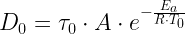
Equation 5 shows that the battery lifetime will degrade exponentially with increasing temperature.

Eq. 5	$D=\tau \cdot A\cdot {{e}^{-\frac{{{E}_{a}}}{R\cdot {{T}_{0}}}}}$
	${{D}_{0}}={{\tau }_{0}}\cdot A\cdot {{e}^{-\frac{{{E}_{a}}}{R\cdot {{T}_{0}}}}}$
	$\tau =\frac{{{D}_{0}}}{A}\cdot {{e}^{\frac{{{E}_{a}}}{R\cdot T}}}={{\tau }_{0}}\cdot {{e}^{-\frac{{{E}_{a}}}{R\cdot {{T}_{0}}}}}\cdot {{e}^{\frac{{{E}_{a}}}{R\cdot T}}}$
	$\tau ={{\tau }_{0}}\cdot {{e}^{-\frac{{{E}_{a}}}{R\cdot T\cdot {{T}_{0}}}\cdot \left( T-{{T}_{0}} \right)}}$
	$\tau ={{\tau }_{0}}\cdot {{e}^{-\frac{{{E}_{a}}}{R\cdot T\cdot {{T}_{0}}}\cdot \Delta T}}$

where

? is the battery's lifetime at a temperature of T.
?₀ is the battery's lifetime at a temperature of T₀.
T is the battery temperature for which we require an estimated lifetime.
?T=T-T₀.
D₀ is the total amount of the corrosion chemical reaction required to degrade the battery to failure.
D is the total amount of the corrosion chemical reaction for a battery at a temperature of T for a time ?.

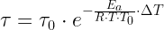
Unfortunately, Equation 5 contains two unknowns (i.e. ?T and T). We cannot directly solve Equation 5 without making an approximation. If we are only interested in temperatures near our reference temperature (T₀), we can say that ${{T}_{1}}\approx {{T}_{0}}\Rightarrow {{T}_{1}}\cdot {{T}_{0}}\approx T_{0}^{2}$ . Equation 6 gives us a useful approximation for the battery's lifetime at a temperature near the battery's reference temperature.

Eq. 6

$\tau \approx {{\tau }_{0}}\cdot {{e}^{-\frac{{{E}_{a}}}{R\cdot T_{0}^{2}}\cdot \Delta T}}$

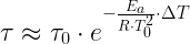Observe that Equation 6 is similar in form to Equation 3:

?T in Equation 5 corresponds to t in Equation 3.
${{\tau }_{0}}$ in Equation 5 corresponds to A₀ in Equation 3.
${{\tau }}$ in Equation 5 corresponds to A in Equation 3.
$E_a / \left( R \cdot T0^2 \right)$ in Equation 5 corresponds to r in Equation 3.
?T is the increase in temperature needed to halve the lifetime of the battery.

Given these correspondences, we can state that the temperature difference required to halve the battery lifetime is given by Equation 7, which is just Equation 3 with the listed substitutions.

Eq. 7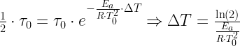

$\frac{1}{2}\cdot {{\tau }_{0}}={{\tau }_{0}}\cdot {{e}^{-\frac{{{E}_{a}}}{R\cdot T_{_{0}}^{2}}\cdot \Delta T}}\Rightarrow \Delta T=\frac{\ln \left( 2 \right)}{\frac{{{E}_{a}}}{R\cdot T_{0}^{2}}}$

Figure 2 provides an example for how the lifetime halving temperature for a typical lead-acid battery is computed.

Figure 1: Temperature Increase that Halves Battery Lifetime.

Figure 2: Temperature Increase that Halves Battery Lifetime.

The calculation in Figure 1 confirms that 10 °C value given here.

Conclusion

I found it interesting that a relationship I have used for years in financial analysis is also useful in battery life calculations. There is something almost magical about the way similar mathematics occurs in very diverse areas.

Save

M	T	W	T	F	S	S
	1	2	3	4	5	6
7	8	9	10	11	12	13
14	15	16	17	18	19	20
21	22	23	24	25	26	27
28	29	30	31

Battery Failure Rates and Continuously-Compounded Interest

Introduction

Background

Chemical Reaction Rates and the Arrhenius Equation

Continuously Compounded Interest

Analysis

Battery Longevity's Relationship to Chemical Reaction Rates

Conclusion

One Response to Battery Failure Rates and Continuously-Compounded Interest

Days Postings

Blog Series

Copyright Notice

Disclaimer