
Talent is God given. Be humble. Fame is man-given. Be grateful. Conceit is self-given. Be careful.
— John Wooden
Introduction

Figure 1: A Motorcycle and Rider Can Be a Projectile (Source).
I recently have had a number of readers ask me to continue my review of Pejsa's "Modern Practical Ballistics". The last major topic I have left to cover is his formula for the drop of a horizontally‑fired projectile as a function of distance. My plan is to derive the formula and present an example of its use. The derivation is not difficult, but it is a bit long and I will divide my presentation into a couple of posts.
This post will examine Pejsa's derivation of the vertical drop differential equation. In my second post, I will examine how he generates both an exact solution and a useful approximate solution that is commonly used in practice. My third post will contain a worked example.
I do not view Pejsa's work as the "state of the art", but it can play a useful role for people who want to develop simple applications for their ballistic work. Pejsa was working at a time when computers had limited capability and people were desperate for simple algebraic methods for getting answers. I consider his work the ultimate expression of the original empirical work done by Mayevski and Ingalls back in the 1870s. This work was important to the development of modern gunnery and I have spent a fair amount of time reading through their papers as part of my interest in battleship gunnery.
For those who want a glimpse into modern ballistics methods, please see the work by McCoy.
Background
Approach
I am going to work hard to use Pejsa's notation, which I do not like and he applies inconsistently. However, using his notation will make referring back to his book much less confusing. I will do my best to carefully comment on the role of each equation and how I am using it.
Definitions
- n
- Atmospheric drag at velocities below the speed of sound is often modeled as varying by the square of the projectile velocity. n is a correction term that is used to "fix" this square-law model for transonic and supersonic velocities. Pejsa defines a different n for four common projectile velocity intervals (ft/s):
- n = 0.5 : 1400 ≤ V < 4000
- n = 0.0 : 1200 ≤ V < 1400
- n = -3.0 : 900 ≤ V < 1200
- n = 0.0 : 0 ≤ V < 900
For this 3-part series, I will be focus my examples on the 1400 ft/s to 4000 ft/s interval, but the work applies equally well to the other intervals.
- A
- A is parameter is a proportionality constant that is specific to the projectile in question and relates acceleration to projectile velocity, i.e.
. It will be used in deriving the projectile drop differential equation, but will not play a significant role in its solution.In his book, Pejsa sometimes uses A to represent acceleration. This created some confusion for me as I read the book. In these posts, I will make sure that A is only used to represent the proportionality constant.
- F(x)
- Pejsa refers to F(x) this as the retardation coefficient and has units of distance. He describes his interpretation of the coefficient in the following quote.
One percent of F is distance in which a projectile loses 1% of its speed to air drag.
For a more detailed discussion of physical meaning of F(x), see this post. F(x) and A are related by the formula
, which I will use in the mathematical development to follow.
Conventions/Assumptions
Here are the key conventions and assumptions in Pejsa's analysis.
- lateral distance is measured along the x-axis, which is positive to the right.
- projectile drop is measured along the y-axis, which is positive toward the ground.
This means that projectile drop is positive in the direction of the ground.
- the force of drag (FDrag) as a function of projectile velocity (v) can modeled using powers of velocity (2-n, where n varies with the velocity of the projectile), i.e.
.
Newton showed that the drag on a slow-moving projectile (i.e. less than transonic speed) varies with the square of it velocity. The drag on projectiles moving at transonic and supersonic speeds can be modeled using other powers of velocity. The convention as been to define n as the correction required to the low-velocity, square-law model.
- I use a yellow highlight for key results from Pejsa's book and a green highlight for significant intermediate results.
Analysis
Tools
All the work done here was in Mathcad, which for this post was primarily used as a mathematical editor. I will use its numerical capabilities in my second post on this topic.
Pejsa's Vertical Drop Differential Equation
We are going to derive the following differential equation for the projectile's velocity in the y-direction as a function of distance.
 |
where
- g is the acceleration due to gravity.
- F0 is F(0).
- n is an exponent determined by the projectiles' velocity. n is a constant in certain velocity intervals.
- v0 is the initial projectile velocity.
- A is the retardation coefficient, which is a function of the ballistic coefficient.
- y' is projectile velocity in the y-direction.
Application of Newton's Laws of Motion
Figure 2 shows the Free Body Diagram (FBD) of the projectile and the associated differential equations.

Figure 2: Differential Equation Setup.
Equation 5 in Figure 2 is the differential equation for the projectile drop as a function of time. We want to modify this differential equation so that we can solve for the projectile drop as a function of horizontal distance.
Velocity Versus Horizontal Distance
In Figure 3, I show how Pejsa computes the projectile velocity as a function of distance.

Figure 3: Derivation of Velocity Versus Horizontal Distance.
Derivation of Flat Trajectory, Projectile Drop Differential Equation
Figure 4 shows how to derive Pejsa's differential equation for the drop of a projectile fired on a flat trajectory as a function of horizontal distance x.

Figure 4: Key Differential Equation with Closed-Form Solution.
Equation 11 in Figure 4 is the key result. This form of the differential equation is useful because:
- It gives us projectile drop as a function of distance.
- It will be shown to have a closed-form solution.
- All parameters can be determined using a projectile's ballistic coefficient, which is readily available for different projectiles.
- It can be used over a wide range of projectile velocities by changing the value of n in the equation.
Conclusion
Given the key differential equation, we can generate a closed-form solution in our next post. If you want to know a bit about Arthur Pejsa, here is a Youtube interview with him.
To better understand F(x) and F0, I went to your article at:
https://mathscinotes.com/2013/09/physical-interpretation-of-a-model-parameter/
Thanks for reminding me! I completely forgot that I wrote about it. I put a link to that material in my text.
mathscinotes.
Just a confusion on my part, wouldn't Eq 4 for velocity include a formula for cos(&)?
You are correct that the cos(δ) should have been included. In Pejsa's derivation, he actually never included it because he assumes that the trajectory is flat enough that you can ignore it.
I have added the cos(δ) to my derivation in Figure 2 and explicitly stated that the cos(δ) is assumed to be 1.
Thanks for the catch.
mathscinotes
Pingback: Pejsa Trajectory Midpoint Formula Given a Maximum Projectile Height | Math Encounters Blog
Just a curiosity question, in your Definitions section you mention values that n will take on given a velocity range. Are these "n" for a G1 or G7 or other shape?
Also, thanks for providing a few hours of fun as I dig into Pejsa's formulas. By the way, I've taken a MathLab program for air resistance that I found on the web and modified it to include Perja's atmospheric drag values for n. Here's the link:
http://www.mathworks.com/matlabcentral/answers/43077-numerical-approximation-of-projectile-motion-with-air-resistance
I'm happy to share my modifications if you wish.
Hi Ronan,
One of the many confusing aspects of the book is whether he is talking about the G1 or G7 shapes. Let's start with Figure 4 from Pejsa's book.
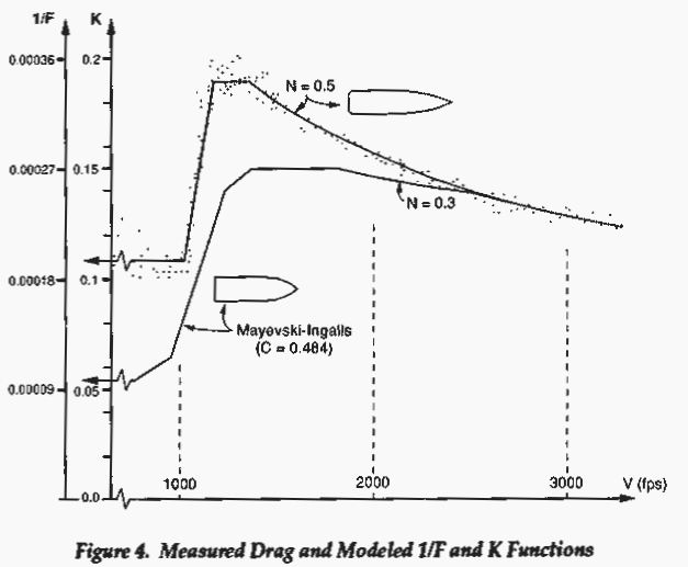
The lower projectile is the G1 reference shape, but with a ballistic coefficient of 0.484. The upper projectile is a US military M2 30 caliber round. For velocities above 2400 fps, these two projectiles have the same drag curve. However, they differ dramatically below 2400 fps.
When Pejsa generated his F curve, he scaled the data for the M2 drag by 0.484. Recall that all this old ballistic data is based on standard projectiles of 1 inch diameter and 1 lb weight. This scaling of the M2 projectile gave him the drag curve for an M2-like projectile relative to the G1 standard projectile (1 inch diameter and 1 lb weight). G7 has not been mentioned anywhere in this discussion. It may be worthwhile putting out a post on this topic. I certainly have all the data in a Mathcad worksheet.
So the Pejsa model uses G1-based ballistic coefficients in formulas that have been fit to the drag curve for an M2-shaped round. What this means is that for typical sporting rounds, use the Pejsa formulas with G1-based ballistic coefficients.
While I went on a bit of a side trip here, this all means that the n's used in the model are not correct for either G1 or G7, but are dead-on for a projectile shaped like a 30 caliber M2 round. This round is similar in shape to a G7, but it is not identical.
mathscinotes
PS
I followed your link and your info looks very interesting. I am pretty tied up now and I will go through it in detail later.
Mark, thanks for the comments and Figure 4. What's nice to know is that the value of n changes depending upon the bullet's velocity, weight and shape.
I tend to think of the 1/F (and drag) as varying with shape and velocity. Drag is a force and the projectile's mass (weight) will affect its rate of deceleration. So a given projectile made of Styrofoam or steel will have the same drag at a given velocity, but the rate of velocity change will be dramatically different.
Just to give you a better feel for how Figure 4 can vary with the projectile shape and velocity, I will also attach the following diagram that shows the coefficient of drag (related to 1/F) for various projectile shapes.
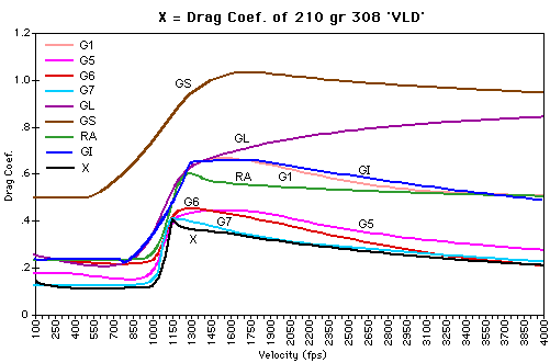
Pejsa's approach can be applied to any of these shapes. It is all a curve fitting exercise.
Notes:
1. I didn't have a idea for the values of Fo and how Pejsa's formula's would compare against a program that takes small time increments to figure out a projectile's position.
2. I found this webpage, http://www.mathworks.com/matlabcentral/answers/43077-numerical-approximation-of-projectile-motion-with-air-resistance, which had MathLab code to figure our a projectile's position with air resistance. The projectile in the code is a baseball.
3. I modified the code to account for Pejsa's v^(2-n) adjustment.
4. I ran this program 3 times considering angles of -10, 0, & 10 degrees.
5. We don't know Fo in advance, so I calculated Fo using the program's calculations for the baseball with velocity v, x, n, and v initial
Program terms:
1. Y Drop = Est Y drop by Pejsa formula - Y calculated by Program
2. RSS Best Fit for Fo is calculated as the best Fo that minimizes:
sqrt(sum((Vi - Vi_est)^2)) where
- Vi is calculated by the MathCad program using time increments of 0.001 seconds
- & Vi_est is calculated by Perja formula for velocity based on initial velocity, x, n and Fo
Initial velocity is: 4000 ft/s
Initial height is: 32.8084 ft = 30 meter
Initial angle is: 0 degrees
Time taken for impact with air resistance is 1.482 seconds. Range is 5271.31 feet.
Time taken for impact without air resistance is 1.42784 seconds. Range is 5711.37 feet.
Statistics data for Calculated Fo
- Max = 23831.12402
- Min = 23822.36395
- Max - Min = 8.76007 <- Very close fit
- Mean = 23826.47868
- Median = 23826.34585
- std = 2.52954
Best RSS Fit Fo 23828.5
Statistics data for Y Drop
- Max = 65.59305
- Min = 0.00000
- Max - Min = 65.59305
- Mean = 22.28483
- Median = 17.02510
- std = 19.66040
Initial angle is: 10 degrees
Time taken for impact with air resistance is 9.713 seconds. Range is 21096.1 feet.
Time taken for impact without air resistance is 89.208 seconds. Range is 351411 feet.
Statistics data for Calculated Fo
- Max = 23292.15890
- Min = 23260.71462
- Max - Min = 31.44428 <-- still close
- Mean = 23267.53719
- Median = 23264.09427
- std = 8.18844
Best RSS Fit Fo 23270.66626 <-- Solved in Excel, Mathlab answer incorrect
Statistics data for Y Drop
- Max = -0.00000
- Min = -1894.09027
- Max - Min = 1894.09027
- Mean = -1420.78204
- Median = -1667.71000
- std = 540.67210
Initial angle is: -10 degrees
Time taken for impact with air resistance is 0.047 seconds. Range is 184.385 feet.
Time taken for impact without air resistance is 46.0455 seconds. Range is 181384 feet.
Statistics data for Calculated Fo
- Max = 23657.98749
- Min = 23657.37379
- Max - Min = 0.61369 <-- extremely close fit
- Mean = 23657.68034
- Median = 23657.68018
- std = 0.18280
Best RSS Fit Fo 23657.8
Statistics data for Y Drop
- Max = 33.27546
- Min = 0.00000
- Max - Min = 33.27546
- Mean = 16.64765
- Median = 16.65292
- std = 9.90547
Mr. Biegert,
While searching last week for the date of Art Pejsa's death I stumbled on your website. I read with great interest two of your posts regarding his work. The rigor you have brought to his work is impressive. I discovered his ballistic work in 2009 as I was looking for an accurate closed form ballistic solution I could use in the field with an HP-35 or HP-42 calculator. Recall that at that time smart phones were not yet widely available and hand held PC's were expensive and not very practical for extended field use. After initial difficulty with his nomenclature I teased a set of equations out of Mr. Pejsa's work which I used the HP-42's very powerful solver function. On 31JUL2009 I discussed with him my interest in building on his work, at which time he gave me "...blanked approval to quote from his work." The HP-42 version matched actual field tests perfectly but soon, smart phones arrived bringing with them the power of Excel, so I developed much more complete ballistic app for long range shooting. A friend and I have tested this app, which I call SmartShot, very thoroughly for eight years including many trips to Africa where we culled nuisance baboons at long range. If you would like to know more about SmartShot please see my web site, projectilescience.com. The following items are posted: a brief overview of SmartShot, a QuickStart manual as well as a detailed manual (still a work in progress), the SmartShot ballistic app itself in htm and several technical notes. We believe the app is easier to use and more accurate, especially deep in the subsonic regime, than traditional apps based on BC's.
You must enter the URL directly into your browser because Google doesn't find it.
I sat down and studied through Art Pejsa's book in two settings. It is a remarkably simple explanation of long range ballistics. Then I put the book back on the shelf of such things and instantly forgot all but the very basics of everything I had learned. I can assure you, long distance records are safe from me. The next week I couldn't have hit a bull in the butt if I'd been swinging a barn door at the target. "Such is our fate, if we live so long ..."
I ordered the disc for PC's; I should have ordered the disc for Mac. If anyone has them, I'd be interested in a trade.
Mr. Biegert,
Three years have passed since I first noticed your interest in Art Pejsa's work. I have continued expand my ballistic app, SmartShot, which is based on his work. The firing solutions, shown on the Products page of my web site, http://www.projectilescience.com, are complete and free to use. My associate and I have demonstrated that Pejsa's math is applicable to all VLD bullets we have tested from 67gn 223 cal to 525gn, 41 cal bullets - in both supersonic and subsonic regimes. SmartShot has been used by the winners of several ELR competitions. Last year preliminary work indicated that Pejsa's equations work with 9mm FMJ pistol bullets.