
Quote of the Day
The road of life is paved with flat squirrels who couldn’t make a decision.
— Source unknown. Indecision is fatal for squirrels. It is also the most destructive management impairment that I can think of.
Introduction
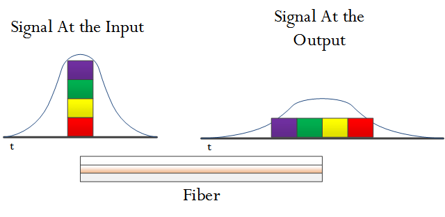
Figure 1: Illustration of Chromatic Dispersion
on a Glass Fiber. A single optical pulse is
composed on a range of wavelengths. Because
each color travels on the fiber with a slightly
different speed, the wavelengths separate as the
pulse travels down the fiber.
The Fiber-To-The-Home (FTTH) market is preparing to make the transition to a data rate of 10 Gigabits Per Second (Gbps) to and from the home. The current Gigabit PON (GPON) standard support 2.5 Gbps to the home and 1.25 Gbps from the home. One of the challenges we are facing with 10 Gbps is managing chromatic dispersion, which is an important optical impairment (see Figure 1).
Transmitting information over a glass fiber requires that we use a laser to modulate the power of the optical signal. To receive the optical signal with a minimum of errors, we need to provide the receiver with (1) an adequate amount of optical power and (2) the bulk of the power for each bit must remain within its assigned bit time. Unfortunately, as the modulated signal travels on the fiber it encounters a number of impairments that reduce its power and spread the power out, which limits the range of the optical system. For PON systems, the most significant impairments are:
- Fiber Attenuation
Every meter of fiber reduces the amount of power in each bit – the losses are mainly from Rayleigh scattering. - Dispersion
Dispersion spreads the power out between bits, causing inter-symbol interference and reduced power for each bit.
In this post, I will be showing how we model the effect of small amounts of dispersion as a power loss. We commonly refer to this power loss at the dispersion power penalty. I will also show how the need to limit the power penalty drives a critical laser parameter, the laser spectral width.
Background
My Quick Description of Chromatic Dispersion
For those who are looking for a quick description of dispersion, I will give you my "elevator pitch" on dispersion in fiber optic communications:
- Different wavelengths of light move at slightly different speeds along a fiber.
- Digital signals are sent on a fiber in the form of pulses of optical power.
- The pulses of optical power are generated by a laser, which produces produces optical power in a narrow range of wavelengths, usually on the order of 0.1 nm.
- As the pulses move down the fiber, the slower wavelengths of light eventually separate from the faster wavelengths of light.
- The separation of the wavelengths as they travel down the fiber causes the pulse to spread out. Eventually, the bits begin to merge together and become impossible to separate. Also, the difference in power between a logic 1 and logic 0 begins to reduce, making it impossible to accurately determine whether a time slot contains a 1 or 0.
Definitions
- Optical Impairment
- Optical fiber is a very good transmission medium, but it is not perfect. It has a number of characteristics that limit its performance, which are referred to as impairments. The usually are broken down into linear and non-linear impairments. Our focus here is chromatic dispersion, which is a very important linear impairment. (Source)
- Chromatic Dispersion
- Dispersion is a physical phenomenon comprising the dependence of the phase or group velocity of a light wave in the medium on its propagation characteristics such as optical frequency (wavelength) or polarization mode. (Source: ITU G.989.2 standard)
- Chromatic dispersion is the result of the different colors, or wavelengths, in a light beam arriving at their destination at slightly different times. The result is a spreading in time of the on-off light pulses that convey digital information. Chromatic dispersion is commonplace, as it is actually what causes rainbows – sunlight is dispersed by droplets of water in the air. In fiber-based systems, an optical fiber, comprised of a core and cladding with differing refractive index materials, inevitably causes some wavelengths of light to travel slower or faster than others. Chromatic dispersion is usually modeled as a combination of material dispersion and waveguide dispersion. (Reference)
- Laser Linewidth
- A spectral line extends over a range of frequencies, not a single frequency (i.e., it has a nonzero linewidth). In addition, its center may be shifted from its nominal central wavelength. (Source)
- Zero-Dispersion Wavelength
- In a single-mode optical fiber, the zero-dispersion wavelength is the wavelength or wavelengths at which material dispersion and waveguide dispersion cancel one another. In all silica-based optical fibers, minimum material dispersion occurs naturally at a wavelength of approximately 1300 nm. (Source)
Wavelengths Used
Figure 2 shows the wavelength plans for the various PON standards. GPON (aka G-PON in Figure 2) is the most common PON type deployed in North America.

Figure 2: Good Summary of the Various PON Wavelength Plans. DS means downstream from the central office. US means upstream to the central office from the homes. PtP means point-to-point and refers to wavelengths dedicated to specific customers. Video refers to the band reserved for NTSC RF video transmissions. (Source)
Dispersion Power Penalty
There are a number of formulas that are used to model the loss of signal power caused by dispersion. For this post, I will be using Equation 1. I chose this formula because it is the most conservative of the commonly used models.
| Eq. 1 |  |
where
- PPD is the dispersion power penalty [dB].
is the spectral standard deviation of the laser [nm].
- B is bandwidth of the signal [Hz].
- L is the length of the fiber [km].
- D is the dispersion constant of the fiber [ps/nm·km].
Equation 1 assumes that the engineer wishes to define the bit time as the period required to contain 95% of the pulse energy at the time of reception. There are lengths that will experience so much dispersion that you will not be able to contain 95% of the pulse energy within the assigned bit time. Mathematically, this means that the expression within Equation 1's logarithm will become zero or negative, which indicates no real solution. I should also make clear that Equation 1 does not model Intersymbol Interference (ISI) – it only models the reduction in bit power.
I like to look at the terms in Equation 1 as shown in Figure 2. I think of dispersion as being a function of two terms: (1) a fiber plant dependent term and (2) a laser transport dependent term.

Figure 3: Breakdown of the Dispersion Power Penalty Formula.
Figure 3 shows a formula with five variables. In the case of G.989.2, the 10 Gbps portion of the standard specifies four of these numbers indirectly as follows:
- B = 10 Gbps
This is the transport data rate and is a fundamental system parameter.
- D · L = 24 ps/nm · 20 km = 480 ps/km
I refer the product of the dispersion constant and the distance as the "dispersion load". It tells you how much delay variance per nm that your system can tolerate. For more information on the dispersion constant, see Appendix A.
- PPD = 0.25 dB (my allotment to dispersion from the total 1 dB power penalty)
There a number of optical impairments that reduce the effective power of the transport.
Given these values from the G.989.2 standard, we can determine our laser's maximum allowed spectral width – the objective of this post.
Analysis
Laser Spectra Width Requirement Derivation
Figure 4 shows how I can determine the required laser spectral width assuming the values for B, L · D, and PPD from the ITU specification. The laser spectral width is normally specified in terms of its Side-Mode Suppression Ratio (SMSR) value. We relate the SMSR value, Δλ, to the σλ using the formula Δλ = 6.07 · σλ. Another common measure of spectral width, Full-Width at Half Maximum (FWHM), has a different conversion factor.

Figure 4: Laser Spectral Width Determination.
A laser with Δλ=0.1 nm is readily obtainable.
Variation of Power Penalty with Distance
Figure 5 shows how the power penalty for a laser with a 0.1 nm spectral width varies with distance.

Figure 5: Power Penalty Versus Distance.
Conclusion
I was able to determine the required laser spectral width to meet the requirements in the NGPNO2 specification. I then used this spectral width to determine how the dispersion power penalty varies with distance.
Appendix A: Dispersion Constant for SMF-28e Fiber
Figure 6 shows how to determine the dispersion constant SMF-28e using Sellmeier's formula. The model and its constants (S0 and λ0) are given in the SMF-28e datasheet.

Figure 6: Dispersion Constant Versus Wavelength for SMF-28e.
Veryy interesting details you have remarked, appreciate it for putting up.