
Quote of the Day
People don't care how much you know until they know how much you care.
Analysis

Figure 1: NTC Bead Thermistor. (Wikipedia - Ansgar Hellwig )
I had a job this week that required that I use the Steinhart-Hart equation for modeling a thermistor's resistance versus temperature relationship. The requirement was driven by the customer's need for high accuracy. Most thermistor applications do not demand high accuracy, but this application can tolerate no more than ±0.5 °C of error. This means that I cannot use the β-based thermistor model, which in this application would have an error of more than ±2 °C. This page will show you how how to perform an efficient 3-point calibration using Excel and a bit of matrix math. As a side benefit, I am using this workbook as an example of matrix math in my Excel tutoring at a local library.
Analysis
The Steinhart-Hart thermistor equation is shown in Equation 1.
| Eq. 1 | 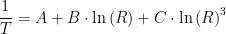 |
where
- A, B, C are calibration parameters.
- R is the thermistor resistance (Ω).
- T is the thermistor temperature (K).
Because there are three unknowns, calibration consists of measuring the thermistor resistance at 3 temperatures and solving the linear system shown in Equation 2.
| Eq. 2 | ![\displaystyle \left[ {\begin{array}{*{20}{c}} 1 & {\ln \left( {{{R}_{1}}} \right)} & {\ln {{{\left( {{{R}_{1}}} \right)}}^{3}}} \\ 1 & {\ln \left( {{{R}_{2}}} \right)} & {\ln {{{\left( {{{R}_{2}}} \right)}}^{3}}} \\ 1 & {\ln \left( {{{R}_{3}}} \right)} & {\ln {{{\left( {{{R}_{3}}} \right)}}^{3}}} \end{array}} \right]\cdot \left[ {\begin{array}{*{20}{c}} A \\ B \\ C \end{array}} \right]=\left[ {\begin{array}{*{20}{c}} {\frac{1}{{{{T}_{1}}}}} \\ {\frac{1}{{{{T}_{2}}}}} \\ {\frac{1}{{{{T}_{3}}}}} \end{array}} \right]](https://s0.wp.com/latex.php?latex=%5Cdisplaystyle+%5Cleft%5B+%7B%5Cbegin%7Barray%7D%7B%2A%7B20%7D%7Bc%7D%7D+1+%26+%7B%5Cln+%5Cleft%28+%7B%7B%7BR%7D_%7B1%7D%7D%7D+%5Cright%29%7D+%26+%7B%5Cln+%7B%7B%7B%5Cleft%28+%7B%7B%7BR%7D_%7B1%7D%7D%7D+%5Cright%29%7D%7D%5E%7B3%7D%7D%7D+%5C%5C+1+%26+%7B%5Cln+%5Cleft%28+%7B%7B%7BR%7D_%7B2%7D%7D%7D+%5Cright%29%7D+%26+%7B%5Cln+%7B%7B%7B%5Cleft%28+%7B%7B%7BR%7D_%7B2%7D%7D%7D+%5Cright%29%7D%7D%5E%7B3%7D%7D%7D+%5C%5C+1+%26+%7B%5Cln+%5Cleft%28+%7B%7B%7BR%7D_%7B3%7D%7D%7D+%5Cright%29%7D+%26+%7B%5Cln+%7B%7B%7B%5Cleft%28+%7B%7B%7BR%7D_%7B3%7D%7D%7D+%5Cright%29%7D%7D%5E%7B3%7D%7D%7D+%5Cend%7Barray%7D%7D+%5Cright%5D%5Ccdot+%5Cleft%5B+%7B%5Cbegin%7Barray%7D%7B%2A%7B20%7D%7Bc%7D%7D+A+%5C%5C+B+%5C%5C+C+%5Cend%7Barray%7D%7D+%5Cright%5D%3D%5Cleft%5B+%7B%5Cbegin%7Barray%7D%7B%2A%7B20%7D%7Bc%7D%7D+%7B%5Cfrac%7B1%7D%7B%7B%7B%7BT%7D_%7B1%7D%7D%7D%7D%7D+%5C%5C+%7B%5Cfrac%7B1%7D%7B%7B%7B%7BT%7D_%7B2%7D%7D%7D%7D%7D+%5C%5C+%7B%5Cfrac%7B1%7D%7B%7B%7B%7BT%7D_%7B3%7D%7D%7D%7D%7D+%5Cend%7Barray%7D%7D+%5Cright%5D&bg=ffffff&fg=000&s=0&c=20201002) |
Because my customer is Excel-focused, I solved this problem in Excel. The workbook is straightforward to use:
- Adjust the columns "Temperature (°C)" and "Mfg Spec (Ω)" to match the manufacturer's thermistor specifications for temperature versus resistance.
- Select the desired calibration temperatures. The resulting maximum error is displayed.
- The spreadsheet calculates the A, B, and C coefficients needed for using this specific thermistor.
My spreadsheet is available here. The thermistor included in the spreadsheet was an arbitrary choice for use as an example.
I understand why you wanted to use excel, but I always enjoy using mathcad for thermistor equations because I can not only fit data to the thermistor equations, but can model the bridge/linearization resistor circuit responses so easily. In particular you can use a find /Minerr block with carefully chosen added points to bias the linearization fitting for a chosen part of the range. Often for medical or biological systems you want best performance around body temperature but need to cover a much wider display range.
One of the cheapest ways to get a really high precision NIST traceable temperature sensing standard is to buy a Calibrated Thermometrics (Now owned by Amphenol I think) Aged glass bead Thermistor Probe where they provide calibration Steinhart-Hart coefficients as well as a 10mC incremental R-T printout and you just use your lab quality 6.5 digit DMM.
Complementary way is few lines of python/sympy...
from sympy import *
var('R1 R2 R3')
var('T1 T2 T3')
var('A B C')
#Ametherm DG103395
T1,R1 = 273.150,31991.6
T2,R2 = 323.150, 3641.0
T3,R3 = 373.150, 686.2
equations = [
Eq( A + B*ln(R1) + C*ln(R1)**3 , 1.0/T1 ),
Eq( A + B*ln(R2) + C*ln(R2)**3 , 1.0/T2 ),
Eq( A + B*ln(R3) + C*ln(R3)**3 , 1.0/T3 ),
]
print solve(equations, (A,B,C))
result is: {C: 1.26349943638314e-7, B: 0.000227813584600384, A: 0.00115679797363983}