Optical Fiber Dispersion Formula - Where Did This Come From?

Quote of the Day

I can calculate the movement of the stars, but not the madness of men.

— Isaac Newton after he lost his shirt in the South Sea Company financial bubble. He claimed to have lost over £2.4 million in today’s money. Arguably history's smartest person, even Newton could not foresee a financial meltdown.

Introduction

Figure 1: Corning Dispersion Equation from SMF-28e Specification.

Most Fiber-To-The-Home (FTTH) deployments in North America use SMF-28e fiber from Corning, which is to fiber what Kleenex is to tissue. Unfortunately, I am so familiar with this particularly product that I can recite its specifications from memory. However, there is one aspect of SMF-28e's datasheet that I have never really understood – the chromatic dispersion formula shown in Figure 1. This formula is used to determine the fiber parameter D(λ), which specifies the travel time difference (in picoseconds [ps]) for photons that differ by 1 nm in wavelength over 1 km of fiber. Dispersion is important because an optical pulse on a fiber is made up of a range of wavelengths that will spread out as they travel down the fiber. Over a long length of fiber, this pulse spreading makes an optical signal undetectable. Dispersion sets the range limit for many fiber-based communication systems.

While looking for other fiber information, I stumbled across the rationale behind this formula and I thought I would write it down here. Let's dig in ...

Background

For general information on dispersion, the best general reference is the Wikipedia. I also have a three-part blog post on the subject.

For those who are looking for a quick description of dispersion, I will make a few points here:

• different wavelengths of light move at slightly different speeds along a fiber.
• digital signals are sent on a fiber in the form of pulses of optical power.
• the pulses of optical power are generated by a laser, which produces produces optical power in a narrow range of wavelengths, usually on the order of 0.1 nm.
• as the pulses move down the fiber, the slower wavelengths of light eventually separate from the faster wavelengths of light.
• the separation of the wavelengths causes the pulse to spread out and eventually become impossible to detect.

Analysis

Empirical D(λ) Characteristic

Figure 2 shows D(λ) for optical fiber like SMF-28e. This figure defines two variables: (1) λ₀, the zero-dispersion wavelength; (2) S₀, the slope of the dispersion characteristic at λ₀.

Figure 2: D(λ) Versus λ for Common Fiber Types.

The Corning formula of Figure 1 uses λ₀ and S₀ from Figure 2 to provide us with a means of computing D(λ).

What is D(λ)?

Fiber optic systems run into problems when a significant percentage of their optical power arrives at the receiver at a different time than the rest of the optical power. We begin by deriving the transit time for light of different wavelengths over a unit length of fiber (Figure 3).

Figure 3: Definition of Transit Time Over a Unit Length of Fiber.

Figure 3 shows that transit time of light over a unit length of fiber is a scaled version of n(λ), the index of refraction for the glass in the fiber.

Using the argument of Figure 3, let's define the D(λ) coefficient as shown in Equation 1.

Eq. 1

where

• D(λ) is the dispersion coefficient at a wavelength of λ.
• n(λ) is the index of refraction of the fiber at a wavelength of λ.
• c is the speed of light in a vacuum.

Index of Refraction Modeling

During my investigation, I was floored at all the different approaches that have been taken for modeling the index of refraction (here is a nice summary). All of these approaches are empirical curve-fits based in some way on the Cauchy , Sellmeier , or Kettler-Helmholtz-Drude equations. Corning mentions in one of their documents that they used Sellmeier's equation. I would argue that they used a simplification of Sellmeier's equation known as Herzberger's equation, which models the index of refraction using the Laurent series shown in Equation 2.

Eq. 2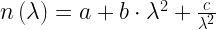

where

• a, b, and c are curve fitting parameters.

Derivation of the Corning Equation

We can derive Corning's dispersion formula by substituting Equation 2 into Equation 1. This equation allows us to compute D(λ) for wavelengths in the range of 1200 nm to 1625 nm using λ₀ and S₀ from Figure 2. The derivation is shown in Figure 4. Because I am in a bit of a hurry, I will use the Mathcad symbolic engine for the derivation, which allows me to just insert a screen capture.

Figure 4: Detailed Derivation of Corning Equation.

Figure 5 shows a plot of the Corning dispersion formula.

Figure 5: Plot of the Corning Dispersion Formula.

Conclusion

This was a nice application of some elementary calculus to the derivation of a formula that optical engineers routinely use.

This derivation also allows us to physically interpret the formulas used to model dispersion. Engineers typically model the effect of dispersion using equations that are functions of (D₀= D(λ₀), L= fiber length, σ_λ= wavelength spread of the laser). We can interpret this term as follows.

Eq. 3

This term represents the amount of time variation we will see in our light pulse over that length of fiber.

Save

Save