My New Cabin Construction

Quote of the Day

The benefit of controlling a modern state is less the power to persecute the innocent, more the power to protect the guilty.

- David Frum


Scope

A number of folks have asked that I post pictures of my cabin construction project. The project actually consists of two separate activities: a large garage (started last fall) and a two-story cabin. I will start posting photos here as things progress.

Old Cabin Demise

The process really began in earnest with the demolition of the old hunting shack that was built in the 1930s.

Figure 1: Old Cabin Demolition.

Figure 1: Old Cabin Demolition.

Garage

The garage is a 30'x60' Morton building. All the garage photos were taken from tree-mounted remote camera. The garage has a storage area, office, and woodshop. I will take more pictures this weekend. Initially, some of my friends suggested that I look for garage alternatives like a Quonset hut or a Carport. These are, of course, quite easy and cost-effective, but I had various needs with a garage, so I decided against it.

Figure 1: Garage Excavation.

Figure 2: Garage Excavation.

Figure 1: Garage Framing.

Figure 3: Garage Framing.

Figure 2: Framed Garage.

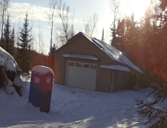
Figure 4: Framed Garage.

The garage contains three rooms: (1) an office with a bathroom and shower, (2) a woodshop, and (3) a boat storage area. You can see the framing in Figure 5. HVAC installation is in progress. Electrical wiring and plumbing will follow. As you can see, there's plenty of storage space. But I still need to build cupboards to keep the outdoor extension cords, lawnmowers, and other tools safe. I might also have to consider getting a new garage air compressor because a lot of heavy work depends on it.

Figure 5: Garage Internal Framing.

Figure 5: Garage Internal Framing.

House

The house is ~2000 square feet and will be my retirement home.

Wow! I never thought I'd say these words because, truthfully, I never thought it would happen. Like most people, I always thought that I'd spend my golden years at the property I'm in now but it is time for a change. A new chapter in a new home sounds good to me. Of course, there are a lot of things that will need renovating before I will be able to move in for good but I'm excited by the prospect. Who wouldn't be?

Though a lot of things need completing in the interior, I also want to place particular focus on the exterior too. After all, this is the first thing that most people will see when they come onto the property. My friend has the same thought process as me and has made the exterior of his home the main priority for his project. Like me, he also loved the idea of a concrete patio, and has since got in touch with somewhere like this Milwaukee Concrete Patio Installation company to see about getting it done for him. At least this way it can be done professionally. I think I will do the same when I finally get around to it.

This is where I'm spending my retirement years, so it just has to be perfect. I have a lot of ideas that I can't wait to turn into a reality. And the best thing is that you're coming along for the journey. Even better! You'll get to see the finished product just as it's been done. And that is very exciting.

Figure 6: Cabin From Driveway.

Figure 6: Cabin From Driveway.

Figure 7: Stamped, Stained, Concrete Patio.

Figure 7: Stamped, Stained, Concrete Patio.

Figure M: Southern Exposure of Cabin.

Figure 8: Southern Exposure of Cabin.

Figure M: Garage and Septic Field from Driveway.

Figure 9: Garage and Septic Field from Driveway.

Save

Save

Save

Save

Save

Save

Save

Save

Save

Save

Save

Save

Save

Save

Save

Save

Save

Save

Save

Save

Posted in Construction, Personal | 10 Comments

Analysis of 555-Based PWM Circuit

Quote of the Day

It is impossible for a man to learn what he thinks he already knows.

— Epictetus, Discourses, Book II Ch.1. This quote caused my career to flash before my eyes.


Introduction

Figure 1: 555 Timer Circuit Causing Analysis Issues.

Figure 1: 555 Timer Circuit Causing Analysis Issues.

I received a request for design formulas that can be used to estimate the frequency (f) and duty cycle (DC) generated by the 555 timer-based, Pulse Width Modulator (PWM)  circuit shown in Figure 1. The presence of diodes in the charge and discharge paths are the main cause of the confusion.

In this post, I will provide: (1) analytic expressions for both f and DC, (2) a detailed derivation of these expressions using Mathcad, (3) an LTspice simulation illustrating how potentiometer resistance affects f and DC, and (4) an error analysis showing the quality of the relationship between the design formulas and the simulation.

As I have mentioned in other posts, I am busy building a cabin and large workshop in northern Minnesota. This means my post will include limited explanatory information because my time is limited.

For those who are interested in my source, my files are here.

Background

Equation 1 can be used to compute oscillation frequency (f) of the circuit of Figure 1 (component locations are defined in Figure 3).

Eq. 1 \displaystyle f=\frac{1}{{{{C}_{1}}\cdot \text{ln}\left( {\frac{{2\cdot {{V}_{{CC}}}-3\cdot {{V}_{D}}}}{{{{V}_{{CC}}}-3\cdot {{V}_{D}}}}} \right)\cdot \left( {{{R}_{2}}+{{R}_{3}}+{{R}_{{POT}}}} \right)}}

where

  • f is the oscillation frequency.
  • RPOT represents the total potentiometer resistance.
  • R2R3, and C1 are passive component values defined in Figure 3.
  • VD is the diode voltage.
  • VCC is the supply voltage.

Equation 2 allows you to compute the duty cycle (DC) as a function of resistance.

Eq. 2 \displaystyle DC=\frac{{{{R}_{2}}+{{R}_{{POT}}}\cdot k}}{{{{R}_{2}}+{{R}_{3}}+{{R}_{{POT}}}}}

where

  • k represents the potentiometer's normalized wiper position, i.e. k ranges from 0 to 1, inclusive.

Notice how Equations 1 and 2 allow you to set the frequency and DC independently. First, set your duty cycle by selecting your resistors, then set your frequency by picking the corresponding capacitor.

Analysis

Formula Derivation

Figure 2 shows my derivation of Equations 1 and 2 using Mathcad 15. There are a couple of things to notice about the formulas:

  • The forward voltage of the diode only affects the oscillation frequency.
  • The duty cycle is a function of the resistances and the potentiometer wiper position.
Figure 2: Derivation of the PWM Formulas.

Figure 2: Derivation of the PWM Formulas.

Simulation Work

I wanted to simulate the circuit in a way that did not require the use of special libraries – like the potentiometer library or a cleaner 555 symbol. Instead, I decided to use two resistors with values that vary in the same manner as the resistance in a potentiometer. Using this approach, I could then created a "wiper" that varied with time, i.e. \displaystyle k=\frac{{time}}{{\left\{ {tTot} \right\}}}, where {tTot} is the total simulation time.

I also used the standard 555 symbol, even though I do not like the way this symbol connects to other parts on a schematic (Figure 3). Yes – I am a bit of a schematic artist.

Figure 2: LTspice Implementation of the 555 PWM Circuit.

Figure 3: LTspice Implementation of the 555 PWM Circuit.

Figure 4 shows the simulation result. As you can see, duty cycle varies as the "wiper" position is changed, i.e. time advances. As expected from Equation 1, the oscillation frequency holds constant as the wiper position is varied.

Figure 3: Output Voltage Simulation For the Circuit of Figure 2..

Figure 4: Output Voltage Simulation For the Circuit of Figure 2. I am only showing part of the simulation because the fine detail is lost at larger scale.

Error Analysis

Figure 5 shows ten data points for which I computed the frequency (Equation 1) and duty cycle (Equation 2) using Mathcad and LTSpice. The agreement is reasonable.

Figure 4: Comparison of Equations to Simulation.

Figure 5: Comparison of Equations to Simulation.

Conclusion

This post derived a pair of formulas that can be used to design a simple, potentiometer-controlled, PWM circuit. The derivation showed good agreement with a Spice simulation of the same circuit.

Posted in Electronics | 1 Comment

Visualizing US vs IJN Aircraft Carrier Numbers During WW2

Quote of the Day

The world may think you are only one person. But to one person, you may be their world.

— Author Unknown. When my children were small, I knew my wife and I were their whole world. This is a big responsibility. Even with adult children, the role of parent is still important – it is the world's best job.


Figure 1: Deployed Carrier Numbers Versus Time During WW2.

Figure 1: Deployed Carrier Numbers Versus Time During WW2.

I watched an interesting lecture on American History TV this weekend called Japanese Perspective on the Battle of Midway by Anthony Tully. The most interesting part of the discussion occurred when Tully began showing how the US production of aircraft carriers eventually overwhelmed the Japanese ability to build carriers. He used some simple graphs to show the relative carrier strength of the US Navy versus the Imperial Japanese Navy (IJN) over time. In this post, I will come up with my own graphics to visualize this information.

It happens that I am taking a course in Excel dashboards right now, and I thought I would try to create my own graphic for this data using some of the techniques shown in this class. To generate the graphic, I needed data. I quickly checked the Wikipedia and it turns out it has a list of WW2 carriers, their date of commission, and date of demise. This data allowed me to generate Figure 1, which I find a bit easier to digest than the graphics shown in the lecture.

Figure 1 shows how US carrier production swamped the ability of the IJN to replace their losses. There are some definitions that are useful in understanding Figure 1.

Aircraft Carrier
Also called a fleet carrier, this was the largest and most capable aircraft carrier type during WW2. (Link)
Light Aircraft Carrier
A carrier design based on cruiser hulls, which resulted in a high-speed design with a complement of aircraft only one-half to two-thirds the size of a full-sized fleet carrier. These carriers filled a gap in fleet protection that existed until more fleet carriers were built. (Link)
Escort Carrier>
A carrier design focused on protecting merchant convoys from submarine attack and provide support to amphibious forces during landings. Escort carriers are generally smaller and slower than fleet or light carriers (Link).

For those who are interested in the details, here is the spreadsheet.

Posted in History Through Spreadsheets, Military History | Comments Off on Visualizing US vs IJN Aircraft Carrier Numbers During WW2

Coal Production By State

Quote of the Day

Learn to love the struggle — if you can’t enjoy the pains of programming, you’re going to face all the more difficulties when you advance to complex problems.

— Joe Previte on learning to program. His statement is true for most other difficult human activities as well. I have heard military folks say that you must "embrace the suck," which is said in a similar spirit.


Figure 1: Wyoming Dominates US Coal Production.

Figure 1: Wyoming Dominates US Coal Production.

I have been listening to politicians discussing US energy policy the last few days. Very few facts were presented during these discussions, but one politician did casually mentioned that Wyoming produces more coal than the next six states combined. I did not know that Wyoming was such a dominating coal producer, and I began to look at how to fact check this statement. Fortunately, the US Energy Information Administration (EIA) has all the data readily available from this web page.

I downloaded the US coal production data from the EIA web page, processed it using Power Query, and created Table 1. I was able to confirm that Wyoming's coal production exceeds the total output of the next six largest coal coal producing states. For those who are interested, here is my Excel workbook.

Posted in Fact Checking | 6 Comments

Linear Temperature Coefficient Resistor Nonlinearity

Quote of the Day

Having proper motivation and honesty are the keys to overcoming fear or anxiety. Fearless and honest self-appraisal can be a powerful weapon against self-doubt or low self-confidence.

— Dalai Lama


Introduction

Figure 1: Resistance Variation with Temperature of a Real "Linear" Temperature Coefficient Resistor.

Figure 1: Resistance Variation with Temperature of a Real "Linear" Temperature Coefficient Resistor.

Our products contain many analog circuits, and these circuits often require temperature compensation in order to meet their requirements across the product's entire temperature range. To perform this compensation, we often use resistors with a specified Temperature Coefficients of Resistance (TCR). A vendor recently stopped manufacturing one of the resistors we use for temperature compensation, and we needed to find a substitute. While searching for a substitute resistor, I needed to understand just how linear the approved resistor's temperature variation is so I can find an appropriate substitute.

Unfortunately, the original designer (gone for over ten years) used a TCR for which the vendor supported but had not published resistance versus temperature curves. The vendor did provide resistance curves for three similar temperature coefficients, which allows me to use interpolation to estimate the curves for the value we are using. Of course, I am requesting that the vendor send me the correct curve. In the meantime, I am just going to interpolate between the specified curves for a preliminary result.

Figure 1 shows my plot of:

  • resistance versus temperature curves for two different TCRs (3900 ppm/°C and 1500 ppm/°C)
  • my interpolated resistance versus temperature curve for a TCR of 3300 ppm/°C.

You can see that there is a small error between the linear ideal and reality. I need to find a substitute part with a similar level of nonlinearity. This post is about viewing the nonlinearity – selecting the substitute part is another matter.

Background

Model for Resistance Variation with Temperature

Equation 1 shows the formula for the variation in resistance for a linear temperature coefficient (i.e. constant TCR) resistor.

Eq. 1 \displaystyle R\left( T \right)={{R}_{{ref}}}\cdot \left( {1+\alpha \cdot \left( {T-{{T}_{{ref}}}} \right)} \right)

where

  • R(T) is the resistor's resistance at a temperature of T.
  • Rref is the resistor's resistance at a temperature of Tref.
  • Tref is temperature at which the resistor's nominal resistance is specified.
  • α is the resistor's TCR.

In Figure 1, I used Equation 1 as my ideal temperature function.

Approach

My analysis approach is simple:

  • Digitize the vendor's three resistance plots (TCRs = 1550, 2700, and 3900 ppm/°C) using Dagra.
  • Perform a two-dimensional interpolation to estimate the response for a TCR = 3300 ppm/°C.
  • Plot  both the ideal and the interpolated responses for a visual comparison of the level of nonlinearity.

Analysis

The analysis was performed in Mathcad and is best viewed either in the Mathcad source or viewing the PDF, both of which are included here.

Conclusion

I am surprised at the typical level of nonlinearity that I am seeing for these resistors. I have always thought that the temperature coefficient for these devices would be a constant, but there is a significant nonlinear component.

Posted in Electronics | 1 Comment

An Intimidating Interview

Quote of the Day

Good programmers comment their code. Great programmers tell you why a particular implementation was chosen. Master programmers tell you why other implementations were not chosen.

— I saw this rule of thumb for commenting code on Stack Overflow. This statement made me think hard about how I comment my code. I see so many comments that tell me what the code is doing and not why – I never seem to have enough why information.


Figure 1: Edward Teller, Father of the H-Bomb. (Source}

Figure 1: Edward Teller, Father of the American H-Bomb. (Source}

I have been reading the book Building the H Bomb: A Personal History by Ken Ford. A major character in the book is Edward Teller, a very famous physicist who is best known as the father of the American H-bomb. I had to smile as I read about Edward Teller. When I worked at Hewlett-Packard, an electrical engineer named Russ Price talked about interviewing for a job at Lawrence Livermore National Laboratory, where he walked into a room and faced Edward Teller as his interviewer. He and Dr. Teller then proceeded to have a very technical interview.

Russ was not familiar with Teller's background, which was probably a good thing. Russ said the interview was pretty tough, but he had nothing but nice things to say about Dr. Teller. He did mention being asked to work a problem about modeling the behavior of a pencil standing on its tip, which he did not know how to solve. Russ also commented that Dr. Teller was very quick and very smart. Unfortunately, Russ did not get the job.

I think I would have turned into a babbling idiot upon seeing him – good thing Russ did not know who Dr. Teller was until after the interview was over.

Save

Posted in Management | 4 Comments

Recoil Calculation Example

Quote of the Day

You have not yet begun to consider what sorts of people are these Athenians whom you may have to fight.

— Thucydides, describing a statement by an ambassador from Corinth who was speaking to the Spartan Assembly. The Spartans were bent on war. This quote is similar to Yamamoto's often cited (but unconfirmedwarning to the Japanese government about going to war with the United States.


Introduction

Figure 1: A-10 Firing its GAU-8. (Source)

Figure 1: A-10 Firing its GAU-8. (Source)

I have been reading about the US Air Force's battle to retire the A-10 Warthog (Figure 1). The USAF has never cared for the A-10 and has made a number of attempts to replace it with either the F-16 or the F-35. During my reading, I saw the following statement about the recoil of its 30 mm Gatling gun, and the impact of this recoil on the A-10's speed.

The average recoil force of the GAU-8/A is 10,000 pounds-force (45 kN), which is slightly more than the output of one of the A-10's two TF34 engines (9,065 lbf / 40.3 kN each). While this recoil force is significant, in practice a cannon fire burst only slows the aircraft a few miles per hour in level flight.

In this post, I will examine these two statements mathematically to determine if I understand them.

Background

Key Performance Parameters

Figure 2 shows the GAU-8 data as stated on the General Dynamics web page.

Figure 2: GAU-8 Key Performance Parameters. (Source)

Figure 2: GAU-8 Key Performance Parameters. (Source)

GAU-8 and Its Projectile

Figure 2: Three Types of 30 mm GAU-8 Rounds. (Source)

Figure 3: Three Types of 30 mm GAU-8 Rounds. (Source)

Figure 3 shows the GAU-8's 30 mm projectile. For this exercise, I will assume the projectile has the following characteristics:

  • Projectile velocity: vMuzzle = 3400 feet per second (fps)
  • Projectile mass: mGAU8 = 395 grams
  • Rate of fire: r = 6000 round per minute

The GAU-8 can be programmed for different rates of fire. I will assume a 6000 rounds per minute for the maximum rate of fire, which will generate the maximum recoil. I will also assume that the gun is fired in burst of 100 rounds, a number that I am guessing based on the ammunition capacity of 511 rounds. Effectively, I am assuming that the gun only has five bursts available.

To estimate the impact of firing the GAU-8 on the speed of the A-10, I will assume that the A-10 weighs 51,000 pounds, which is its listed maximum takeoff weight.

Analysis

Shortcomings of this Analysis

No explosion-driven device is 100% efficient at converting chemical energy into projectile energy. In the case of gun, it is common to assume that as much as 20% of available powder energy goes into the gases that escape from the end of the barrel. I do not know the impact of this gas discharge on the overall recoil for a GAU-8, but it is significant. I will ignore this escaping gas in my analysis below, which means that my calculations provide a lower bound on the recoil of this weapon.

In reality, recoil can only be accurately estimated with detailed knowledge of the gas discharge characteristics.

Recoil Analysis

Figure 4 shows how to estimate the amount of recoil by assume that recoil is do to the change in momentum caused by the opposing momentum of the fired projectiles. Note that this estimate ignores the momentum of the expelled gases.

Figure 3: Recoil Calculation.

Figure 4: Recoil Calculation.

We see that the recoil must be greater than 9,200 pounds, which means that the stated recoil force of 10,000 pounds is reasonable.

Impact on A-10 Speed

Figure 5 shows how you can estimate the reduction in the aircraft's speed caused by the firing of the GAU-8.  I calculate that the impact of the GAU-8 on the A-10's speed is ~4 miles per hours, which roughly agrees with the statement quoted in this post's introduction, i.e. a few miles per hour.

Figure 4: Impact of GAU-8 Firing on A-10 Velocity.

Figure 5: Impact of GAU-8 Firing on A-10 Velocity.

Conclusion

The fact that the GAU-8 has ~5 tons of recoil force is amazing. It is hard to believe a weapon like that can be mounted on an aircraft.

As I worked on this problem, I recalled a Woody Woodpecker cartoon within the movie Destination Moon that illustrated how a firing a rifle can generate thrust.

Figure 6: Woody Woodpecker Explains Newton's Third Law.
Posted in Ballistics, Military History | 2 Comments

Lake Level Variation Over Time

Quote of the Day

If physics was about proofs, von Neumann would be a pretty good physicist.

Wolfgang Pauli, after reading a rigorous mathematical proof about some aspect of quantum mechanics by John von Neumann.

Figure 1: Plot of Eagle Lake Level Relative to Sea Level.

Figure 1: Chart of Eagle Lake Level Relative to Sea Level. The Ordinary High-Water Mark (OHWM) is the level used by the State of Minnesota for determining how far away buildings must be placed from the water.

My wife and I are building a vacation home on the shores of Eagle Lake in Itasca County, Minnesota. We also are active members of the local lake association, which is a group of homeowners who work on projects to keep our lake healthy. One task I perform on a yearly basis for the lake association is to draw a graph of how our lake level is varying over time (Figure 1). The lake level is important to homeowners because it affects the amount of beach that is exposed and the length of their docks.

Figure 1 shows how our lake level has varied since 2001. The peaks correspond to recent heavy rains. The low points tend to corresponds to times when a beaver dam at the lake outflow fails, releasing water,  and causing a quick reduction in lake level. In general, the beavers perform excellent maintenance on their dams, but trappers occasionally remove the beavers, and then the beaver dams fall into disrepair until a new beaver pair arrives. No lake level measurements are taken during the winter because the lake is frozen and covered in snow. I indicate winter in Figure 1 with a snowflake symbol.

I attach my spreadsheet here for those who are interested in how this chart is obtain the lake level information. Power Query is used to grab the data from the State of Minnesota and clean the data up for graphing. I use standard Excel commands for plotting the data.

Save

Posted in Cabin | Comments Off on Lake Level Variation Over Time

Sugar-to-Flour Mass Ratios in Cake Recipes

Quote of the Day

The Hemingway we are talking about did not choose his death.

— Orson Welles, talking about Ernest Hemingway and how he suffered near the end of his life. Hemingway was not the same man at the end of his life that Welles had known earlier.


Introduction

Figure 1: Histogram of Sugar-to-Flour Mass Ratios in 62 Cake Recipes.

Figure 1: Histogram of Sugar-to-Flour Mass Ratios in 62 Cake Recipes.

I have been working at becoming a better baker. Specifically, I have been trying to understand how recipes are developed. Many baker's begin developing their recipe's based on ratios of ingredients. The classic rule ratio of thumb for cake recipes is to use equal masses of flour, sugar, butter, and eggs – with the ingredient ratios expressed as 1:1:1:1.

I recently noticed that many of the recipes that I have been using do not follow this rule of thumb. I was most curious about how the ratio of sugar-to-flour varied between recipes. I found a text database of cake recipes and decide to create a histogram that shows how the sugar-to-flour mass ratio varies.

Background

Flour and Sugar Densities

Recipes in the US tend to use volume measures like cups rather than mass measures. To convert these volume measures to masses, I needed to determine the densities of flour and sugar in terms of cups (Figure 2).

Figure 2: Computing the Density Ratio of Sugar-to-Flour.

Figure 2: Computing the Density Ratio of Sugar-to-Flour.

Confounding Issues

Cake recipes frequently contain ingredients that affect the amount of flour or sugar required. Example of these confounding ingredients include:

  • cocoa (reduces the need for flour)
  • honey (reduces the need for granulated sugar)
  • applesauce
  • candied fruit (e.g. cherries)

Also, the recipes sometimes call out sifted flour, which has a lower density than unsifted flour. For my analysis here, I am ignoring confounding ingredients and just looking at the ingredients labeled sugar and flour (granulated or brown) and taking their mass ratios.

Analysis

My analysis was performed using Excel and Power Query. I have included my analysis and data here. I did not use every recipe in the text database because many recipes had obvious confounding sources of sugar. For example, some recipes had large amounts of sugar added in the form of juices and fruits. I flagged the recipes I used by prefixing their names and their flour and sugar ingredients with "@" symbols. This made it simple to extract the information that I needed.

Once I had extracted the ingredients, I then determined the volume ratios and converted the volume ratios to mass ratios using the densities of flour and sugar.

Conclusion

The 1:1 mass ratio between flour and sugar appears to be violated frequently. In fact, the 1:1 volume ratio between flour and sugar is more common than the 1:1 mass ratio.

Save

Save

Save

Save

Save

Save

Posted in Baking | Comments Off on Sugar-to-Flour Mass Ratios in Cake Recipes

Real-Life Equipment Optimization Problem

Quote of the Day

First forget inspiration. Habit is more dependable. Habit will sustain you whether you’re inspired or not.

Octavia Butler. It is very important to cultivate habits that promote excellence. Jack London used to say that "You can't wait for inspiration, you have to go after it with a club." I believe that as well. I often find that inspiration comes in the quiet times that occur after I have laid siege to a problem for a while.


Introduction

Figure 1: Illustration of the Manufacturing Situation.

Figure 1: Illustration of the Manufacturing Situation.

I recently was asked to provide a recommendation on how to schedule the operating time for three different machines that were producing three different products. This is not a made up problem, but reflects a real production situation. My solution uses Excel's Solver and its linear programming-based optimization routine to find an optimal machine scheduling plan. The solution I provided has proven to be useful to the folks who asked for it, and I thought it was worth sharing my solution here.

I should mention that the model I am showing here is only the first-round of my modeling effort. I am continuing to work with the group that is responsible for this manufacturing effort to create a more detailed model of their manufacturing process. The effort has been very interesting and has provided much insight into their manufacturing process.

For privacy reasons, I have normalized all product costs and have changed all the default values from their true values.

Problem Description

Figure 1 shows a high-level illustration of the manufacturing situation. The following list defines the problem and its constraints:

  • There are three machines called 1, 2, and 3.
  • There are three products being manufactured called A, B, and C.
  • Each product has a different unit market value.
  • We will be be optimizing the total product value produced by these three machines each month.
  • Machine 1 can only produce product A.
  • Machine 2 can only produce product A.
  • Machine 3 can produce either product B or C.
  • Machine's 1 and 3 share the same electrical supply and only one of these machines can be run at a time. I should mention that these machines are enormous, in a remote location, and take a considerable amount of power. Upgrading the electrical service is prohibitively expensive.
  • Machine 3 requires time to switch from producing B to C and vice-versa. I will not be modeling this loss of production – I will include switch-over time in a later model. I needed to get an initial solution out immediately.
  • There are production contracts that mandate that a minimum number of A, B, and C products must be manufactured each month.
  • The machines have a certain amount of downtime that is related to their hours of operation. I have modeled these maintenance operations as a loss of efficiency.

Analysis

I am not going to go through the details of the spreadsheet here in text – I recommend you just look at the spreadsheet itself. Here are its critical features:

  • The spreadsheet uses simple VBA macros to select canned scenarios and run the solver.
  • I have defined four scenarios that you can select using radio buttons.
  • You can change the inputs to whatever you want and click the solve button to generate a custom solution.

Here is my spreadsheet.

Conclusion

The model provided us a very useful discussion vehicle for understanding and evaluating the manufacturing process in terms of:

  • machine efficiency
  • switching time
  • product mix
  • electrical power

While I plan to continue to refine the model, the spreadsheet included here is proving to be quite accurate.

Posted in General Mathematics | 3 Comments